Data table
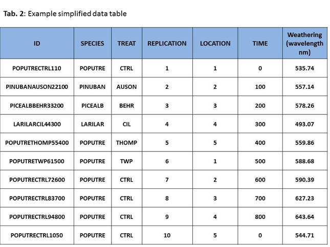
The simplified data table consists of 7 columns (c.f. Tab. 2). The first column on the left side shows the ID concluded named through the following unit columns (Species, Treat, Replication, Location and Time), which create a name like POPUTRECTRL110 in the second row (c.f. Tab. 2).
The unit SPECIES lists the four different Species:
TWP 200 (TWP), BEHR PENETRATING OIL FINISH (BEHR), THOMPSONS TIMBER OIL (TOMP),CIL WOODCARE (CIL), AUSON’S Pine Tars/Stain (AUSON) (c.f. Tab 1. Methods).
The REPLICATION column shows the replication No. of the samples between 1 to 10. The LOCATION column presents the location of the 5 measurement points for the spectrophotometrie – wavelength measurement (c.f. Fig. 2: Laboratory test sample – Methods). The unit TIME lists the different time intervals for the measuring from 0 hours to 800 hours in 100 hour steps. The WEATHERING column shows the measured wavelength in nanometer (nm) for each measurement point.
The simplified data table consists of 7 columns (c.f. Tab. 2). The first column on the left side shows the ID concluded named through the following unit columns (Species, Treat, Replication, Location and Time), which create a name like POPUTRECTRL110 in the second row (c.f. Tab. 2).
The unit SPECIES lists the four different Species:
- Larix larcinia (LARILAR),
- Pinus banksiana (PINUBAN),
- Picea alba (PICEALB),
- Populus tremuloides (POPUTRE)
TWP 200 (TWP), BEHR PENETRATING OIL FINISH (BEHR), THOMPSONS TIMBER OIL (TOMP),CIL WOODCARE (CIL), AUSON’S Pine Tars/Stain (AUSON) (c.f. Tab 1. Methods).
The REPLICATION column shows the replication No. of the samples between 1 to 10. The LOCATION column presents the location of the 5 measurement points for the spectrophotometrie – wavelength measurement (c.f. Fig. 2: Laboratory test sample – Methods). The unit TIME lists the different time intervals for the measuring from 0 hours to 800 hours in 100 hour steps. The WEATHERING column shows the measured wavelength in nanometer (nm) for each measurement point.
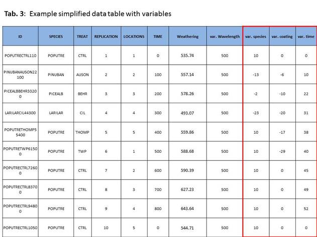
To explain the predictor variables and the response variable it is helpful to have a look on Tab. 3 . The data set and the variables for this project are manipulated, so the predictor variables are easy to identify (red marked). Species, Treatment and Time are the predictor variables in a non-manipulated experiment. In our case this predictor variables are manipulated by the different variable numbers in the columns var. species for the unit Species, var. coating for Treatment and var. time for Time. All variations are based on the var. wavelength of 500 nm. For example, in the third row the variation for the species (PICEALB) is (-2), the variation for the coating (BEHR) is (-10) and for the time of 200 hours is (22).
This three predictor variables based on the wavelength of 500 nm and added by random effect of 60 [RAND*60()] resulting to our weathering response variable. In total we get 8.640 weathering results to analyze.
Exploratory graphics
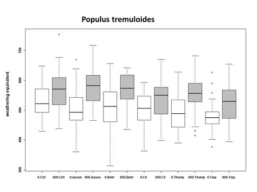
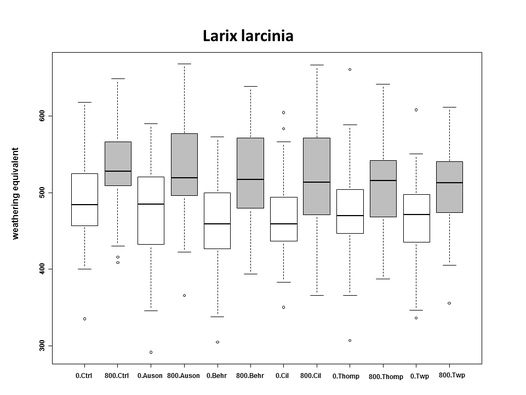
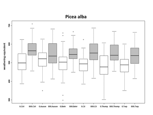
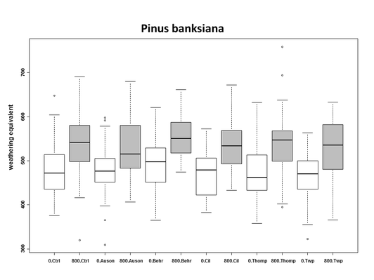
The 4 box plots below for analyzing the data set show the variability of the measurements comparing the 4 different wood species. Two box plots represent the measurements for the different treatments. The white box plot always represents the treatment for the time 0 hours at the beginning of the test. The grey box plot represents the treatment at the end of the test after 800 hours. The box plots among each other show a big variance of different big boxes, whiskers and outliers, which accounts for the high random effect of 60. The distribution of the box plots is totally randomly and not specified on one species or treatment.
The 4 box plots below for analyzing the data set show the variability of the measurements comparing the 4 different wood species. Two box plots represent the measurements for the different treatments. The white box plot always represents the treatment for the time 0 hours at the beginning of the test. The grey box plot represents the treatment at the end of the test after 800 hours. The box plots among each other show a big variance of different big boxes, whiskers and outliers, which accounts for the high random effect of 60. The distribution of the box plots is totally randomly and not specified on one species or treatment.
|
|
|
|
Fig. 3: Box plot comparison of the different treatments at time 0 hours (white plot) and at 800 hours (grey plot) of the weathering for the 4 different wood species
